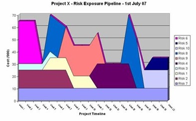
I was looking through the current set of risk presentations on slideshare, and found an interesting one called Creating Risk Profile Graphs, adapted from an article on managing project risks by Mike Griffiths over at the Leading Answers blog. The approach taken is to define and rate project risk factors and then plot their development over time. The graph below (double click for a better view) shows the profile of 10 technology risks over 4 months charted into Excel as "stacked" area graphs. There is another view on the same risk factors here.

The risk factors measured include JDBC driver performance, calling Oracle stored procedures via a web service, and legacy system stability. The project manager rates each risk factor monthly for severity and probability to produce a numerical measure of the risk factor. Plotted over time we see 4 persistent project risks (the steel and light blue, tan and pink plots).
I was not sure if this was a good way to create a risk profile, so I did a Google image search to see what else was out there. The results were very interesting, and reflect the varying approaches risk managers use to present their results.
This first risk graph really leapt off the search page results, if for no other reason than the prominent pink silhouette of Dilbert's manager in the middle. I must confess that the meaning of the graph was not apparent, but luckily its part of an article called Risk Management for Dummies (click and scroll down) where it is explained to be a depiction of the peaks and troughs in the risk exposure pipeline. The graph is tracking the cost of risks over time.
The next profile is a common, if not traditional, format for risks, taken from the integrated risk management guide of the Canadian Fisheries and Oceans department. This is also called a risk rating table, risk map or risk matrix. Likelihood is represented on the horizontal axis and impact (severity) on the vertical axis.

In the first two graphs these two dimensions were combined into a single risk measure (vertical) and then plotted over time (horizontal). The graph above has no representation of time and risks are rated against their current status red, yellow and green regions in the table correspond to measures of high, medium and low risk respectively, and the exact choice of the boundaries is flexible but normally fixed across a company. The table is 5 x 5 but it is also common to have 4 x 4, 5 x 5, 6 x 4, and so on. Below is a 3 x 3 variant of the risk rating table with the high risk region moved to the upper left corner rather than the traditional upper right corner. Note that there is an additional qualitative region and that the regions do not respect the table format. This one is also about fish and oceans, and also from those Canadians but part of another guide.

The risk rating or profile table below is quite close to the format used in my company, taken from a recent annual report of a healthcare company. Again there are the two dimensions of likelihood and severity. There are 6 risks in the table represented by current rating and target rating after mitigation actions have been performed (the arrows show the improvement of each risk). Note that the mitigation of risk 6 yields no improvement, a reasonably common occurence in practice.

Note also that the red, yellow and green have been replaced by different shades of the single colour blue. The colour red has such a strong association with danger that using it in a risk profile is often counterproductive since all attention is drawn to the red region. In the above graph different shades of blue have been used to represent the relative profiles of risks.
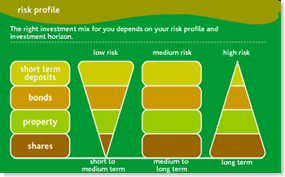
The next risk profile is more graphic than graph, and communicates that concentrating your portfolio in shares is high risk, while short term deposits are low risks. It is taken from an investment article in a newspaper. This graph(ic) is not very sophisticated but it does get its main point across.
The final profile is more quantitative. The graph rates probability against result (impact), which can be positive (upside), neutral or negative (downside). It is from a post on the risk of global warming. In this case the upside seems rather limited while the negative impact tail extends much further. So the profile of this risk is dominated by its downside. The fat tail of the downside is hard to capture in a rating table for example.

Related Post


4 comments:
Very understandable graph I know what you mean thanks for sharing.
Laby[seersucker suit]
Corporate photography demands high levels of professionalism to bring out the best in a person. A winning corporate portrait can be achieved with the required adjustments to make the subject stand out from the surrounding. See more samples of company profile
https://www.roknelbeet.com/نقل-اثاث-بجدة/
https://www.roknelbeet.com/نقل-اثاث-بالدمام/
https://www.roknelbeet.com/نقل-اثاث-بمكة/
https://www.roknelbeet.com/تخزين-اثاث-بالرياض/
شركة مكافحة حشرات بالاحساء
شركة مكافحة حشرات بالخبر
Post a Comment